Chemistry in R
Within pharmaceutical research there is often the need to represent chemical structures. In this blog post, I do a quick tour of the tools available to do so in R.
Two of the projects for representing and manipulating chemical structures in R are rcdk and ChemmineR. Here, I will present how to do basic input, display and output with the two libraries.
Setup
To install rcdk it as as easy as running install.packages("rcdk"). For this to work, rJava needs to be installed. In the off chance
problems arise with the Java version or location the following link provides
useful help on how to solve this issue.
To obtain ChemmineR we need to first install bioconductor by running install.packages("BiocManager") in the console and
then use the install() function within this package to install ChemmineR and
ChemmineOB. If OpenBabel is not installed or issues arise when calling the library function on ChemmineOB please refer to OpenBabel
and follow the installation instructions for the corresponding particular operating system.
install.packages("rcdk")
install.packages("biocManager")
install.packages("webchem")

BiocManager::install("ChemmineR")
BiocManager::install("ChemmineOB", dependencies = T)
After installing the following libraries will be necessary
library(ChemmineOB)
library(ChemmineR)
library(rcdk)
library(here)       # Access files in blogdown
library(fs)         # Access files in your file system
library(webchem)    # Query chemical databases
library(tidyverse)  # Data Superpowers :)
Now we are ready to start representing chemical data in R.
The data formats
Two common data formats for chemical structure representation are SDF and SMILES. Both Structure Data Files and the Simplified Molecular Line Entry System are text files which encode information such as atom connectivity, identity and content. The SDF format consists of 8 parts 1) a block header with a title 2) A count line block, 3) an atom table, 4) a bond table (As shown in the figure below), 5-6) other molecular properties whose line starts with the letter M as well as the END delimiter of the connectivity property block, 7) other properties as key value pairs delimited by a new line and 8) a final delimiter for each compound.
 The header(1) has a title with information regarding the name of the molecule
or some compound identifier (CID) from the database the file was obtained. In
this case it has the PubChem ID for caffeine. The count line block(2) indicates
in the first position how many atoms are there in the molecule and in the second
position how many bonds. The details of the atom’s identity and content are
spelled out in the atoms table(3). In the example above caffeine has 24 atoms and
25 bonds. Along with the atom’s identity the X, Y, Z coordinates for the molecule
are provided, if available, in the first three column of the atoms table (3). Right
below the atoms table one finds the bonds table, which indicates how atoms are
interconnected with one another to form a structure. The first two column in the
bonds table are the from and to connectors in the compound graph and the third
column represents the type of bond: (1) for single, (2) for double and other
special bond types.
The header(1) has a title with information regarding the name of the molecule
or some compound identifier (CID) from the database the file was obtained. In
this case it has the PubChem ID for caffeine. The count line block(2) indicates
in the first position how many atoms are there in the molecule and in the second
position how many bonds. The details of the atom’s identity and content are
spelled out in the atoms table(3). In the example above caffeine has 24 atoms and
25 bonds. Along with the atom’s identity the X, Y, Z coordinates for the molecule
are provided, if available, in the first three column of the atoms table (3). Right
below the atoms table one finds the bonds table, which indicates how atoms are
interconnected with one another to form a structure. The first two column in the
bonds table are the from and to connectors in the compound graph and the third
column represents the type of bond: (1) for single, (2) for double and other
special bond types.
Another popular notation for representing chemical data is the SMILES format. SMILES are another text based representation of a chemical formula. Compare caffeine’s representation in the SDF table file to the SMILES string provided below.
CN1C=NC2=C1C(=O)N(C(=O)N2C)C
The number of atoms in the SDF file and the SMILES format show a total difference in atom number. This difference is not an error, the SMILES format omits hydrogens whereas this particular version of SDF explicitly shows them. Just like with programming languages there are a multiplicity of ways to represent information. The SDF and SMILES are just two of many.
Interconverting between formats would be a hassle. Luckily, machines and programming languages can help us interpreting these formats and handle data at larger scales with much more ease.
Importing chemical data into R
Reading SDF with rcdk
Reading SDF data can be achieved withrcdk via its function rcdk::load.molecules().
The function is quite flexible in that it is able to read both local files as
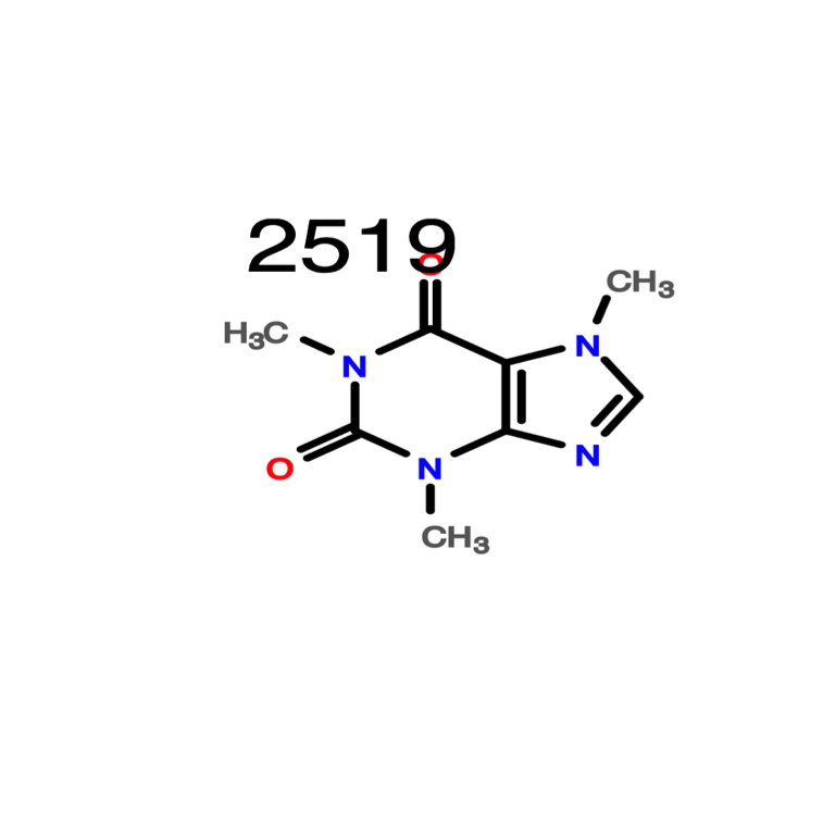
well as remote ones. Here, I am specifying the pubchem SDF link for caffeine and
then using the function view.molecule.2d() to visualize it.
caffeine <- rcdk::load.molecules(
  "https://pubchem.ncbi.nlm.nih.gov/rest/pug/compound/CID/2519/record/SDF/?record_type=2d&response_type=save&response_basename=Structure2D_CID_2519",
  typing = T
  )
ethanol  <- rcdk::load.molecules(
  "https://pubchem.ncbi.nlm.nih.gov/rest/pug/compound/CID/702/record/SDF/?record_type=2d&response_type=save&response_basename=Structure2D_CID_702",
  typing = T
  )
capsaicin <- rcdk::load.molecules(
  "https://pubchem.ncbi.nlm.nih.gov/rest/pug/compound/CID/1548943/record/SDF/?record_type=2d&response_type=save&response_basename=Structure2D_CID_1548943",
  typing = T
  )
rcdk::view.molecule.2d(caffeine)
The view.molecule.2d() will open an applet showing the structure of caffeine.
Display of SDF with rcdk
For inline display of chemical structures as part of the rnotebook a workaround
is necessary. To produce output along with the rnotebook the function
view.image.2d() is used together with plot() and rasterImage() as shown in
the vignette example from rcdk,a solution I first saw at cureffi. Removing the bounding around the plot and setting
the image to the same dimensions as the plot allows for a cleaner presentation
of the molecules. I still have to figure out how to change the background color
in the view.image.2d() function.
plot_molecule <- function(molecule, name = NULL, sma = NULL, ...){
#' molecule an object as returned by rcdk::load.molecules or rcdk::parse.smiles()
#' name a character for the name of the molecule,
#' sma a character witht the smarts string as passed onto get.depictor()
#' ... other arguments for get.depictor()

# Image aesthetics
dep <- get.depictor(
                    width = 1000, height = 1000,
                    zoom = 7, sma = sma, ...
                    )
molecule_sdf <- view.image.2d(molecule[[1]], depictor = dep)


## Remove extra margins around the molecule
par(mar=c(0,0,0,0))
plot(NA,
     xlim=c(1, 10), ylim=c(1, 10),
     # Remove the black bounding boxes around the molecule
     axes = F)
rasterImage(molecule_sdf, 1,1, 10,10)
# Annotate the molecule
text(x = 5.5, y = 1.1,  deparse(substitute(molecule)))
}

plot_molecule(caffeine, abbr = "reagents", annotate = "number", suppressh = T)

Reading and displaying SMILES with rcdk
In the two versions of caffeine presented above the difference between explicit and implicit hydrogens can be readily observed. The atoms in the caffeine structure are numbered according to the order in which they appear in the atoms table in the SDF file. Notice how we can obtain the same results by parsing the SMILES for caffeine.
smiles_caffeine <- parse.smiles("CN1C=NC2=C1C(=O)N(C(=O)N2C)C")
plot_molecule(molecule = caffeine ,
              abbr = "reagents",
              annotate = "number",
              suppressh = F
              )
Functional groups in a molecule can be highlighted by passing the corresponding SMART
string to the get.depictor() function as shown below. An approach that could
be very useful if one is interested in highlighting regions of a molecule
associated with a particular activity.
plot_molecule(caffeine, sma = "c=O", abbr = "reagents")
Writing to file with rcdk
Writing to file with rcdk can be achieved with the write.molecules function. If
provided with a vector of molecules write.molecule() will append them into the same
file.
write.molecules(c(capsaicin, ethanol, caffeine),
                filename = tempfile(pattern = "chili-rum-coffee",
                                    fileext = ".sdf"
                                    ),
                together = T
                )
Reading SDF with ChemmineR
The next library available in R is ChemmineR. We can use the file we saved with rcdk and read it into ChemmineR.
data_sdf <- ChemmineR::read.SDFset(fs::dir_ls(tempdir(),
                                              regexp = "chili-rum-coffee",
                                              recurse = T)
                                   )
What I enjoy about ChemmineR is the capacity to extract specific regions from the SDF with a single function call. Here’s the atom specification section discussed earlier accessed via ChemmineR.
atomblock(data_sdf[2])
## $CMP2
##         C1      C2 C3 C5 C6 C7 C8 C9 C10 C11 C12 C13 C14 C15 C16
## O_1 3.7320  0.2500  0  0  0  0  0  0   0   0   0   0   0   0   0
## C_2 2.8660 -0.2500  0  0  0  0  0  0   0   0   0   0   0   0   0
## C_3 2.0000  0.2500  0  0  0  0  0  0   0   0   0   0   0   0   0
## H_4 2.4675 -0.7249  0  0  0  0  0  0   0   0   0   0   0   0   0
## H_5 3.2646 -0.7249  0  0  0  0  0  0   0   0   0   0   0   0   0
## H_6 2.3100  0.7869  0  0  0  0  0  0   0   0   0   0   0   0   0
## H_7 1.4631  0.5600  0  0  0  0  0  0   0   0   0   0   0   0   0
## H_8 1.6900 -0.2869  0  0  0  0  0  0   0   0   0   0   0   0   0
## H_9 4.2690 -0.0600  0  0  0  0  0  0   0   0   0   0   0   0   0
Likewise, the bond matrix can also be obtained as shown below.
bondblock(data_sdf[2])
## $CMP2
##   C1 C2 C3 C4 C5 C6 C7
## 1  1  2  1  0  0  0  0
## 2  1  9  1  0  0  0  0
## 3  2  3  1  0  0  0  0
## 4  2  4  1  0  0  0  0
## 5  2  5  1  0  0  0  0
## 6  3  6  1  0  0  0  0
## 7  3  7  1  0  0  0  0
## 8  3  8  1  0  0  0  0
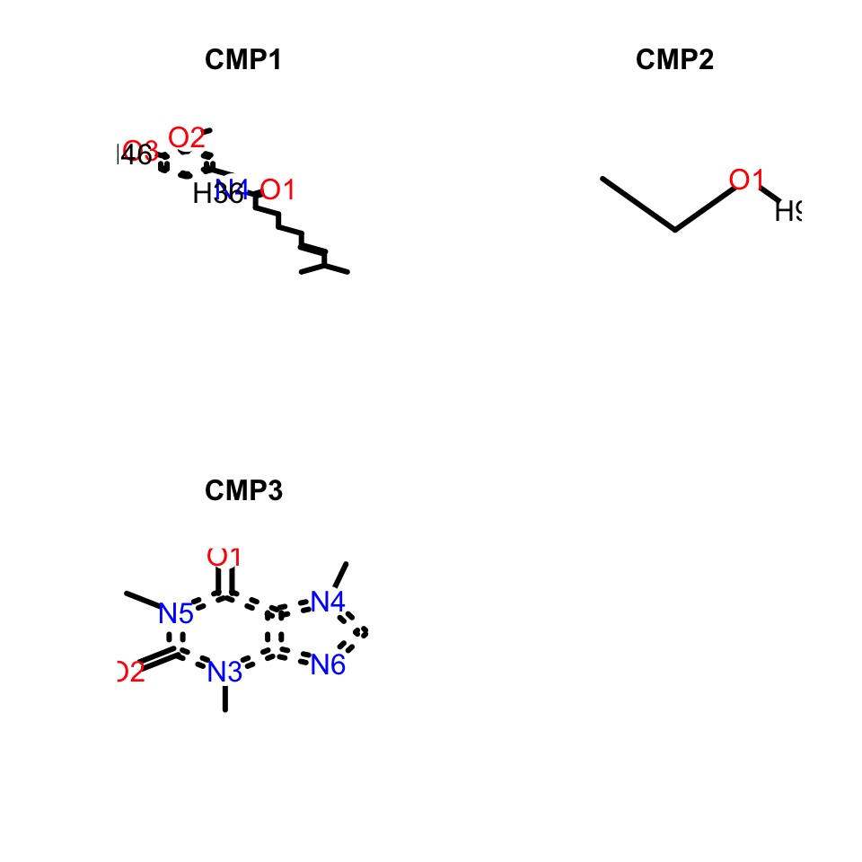
The SDF container in ChemmineR can be passed directly to R’s plot function to visualize the resulting molecule. If multiple SDF are provided a grid with each compound will be provided. Below, I show the structure of capsaicin, the chili pepper molecule.
Display of chemical structures with ChemmineR
plot(data_sdf[1], print = F, atomnum = T)
If the sdf object in ChemmineR is not subsetted the resulting output is a grid with all the molecules present in the object.
plot(data_sdf, print = F, atomnum = T)
Better image quality can be obtained with the openBabelPlot function.
openBabelPlot(data_sdf[3])
Format interconversion is readily accessible from ChemmineR with the aptly named functions sdf2smiles and smiles2sdf.
chemminer_smiles <- data_sdf %>%
  sdf2smiles()
chemminer_smiles
## An instance of "SMIset" with 1 molecules
Writing to file with ChemmineR
Finally output to file in ChemmineR uses write.*() functions. We can save to file our three molecules.
ChemmineR::write.SMI(chemminer_smiles,
                     file = tempfile(pattern = "chemminer_chili-rum-coffee",
                                     fileext = ".txt"))

ChemmineR::read.SMIset(file = fs::dir_ls(tempdir(), regexp = "chemminer", recurse = T))
## An instance of "SMIset" with 1 molecules
With the development of the reticulate package porting functionality from python packages such as RDKit should also be readily accessible from R.
Conclusions
More complex routines can be built with the functions in the libraries mentioned in this post. The vignettes for both ChemmineR and rcdk provide examples of clustering and substructure searches analysis as demonstrations. Often, it all starts with basic input, display and output to get going with the rest of the analysis.